💡 Key Takeaways
- A high Sharpe is not evidence on its own. The Deflated Sharpe Ratio (DSR) corrects a backtest Sharpe for two inflation sources at once: selection bias from trying many strategies, and non-Normal (skewed, fat-tailed) returns.
- The bar moves with the number of trials. Even if the true Sharpe is zero, the expected maximum Sharpe across
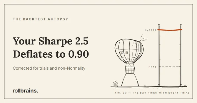
Nindependent trials is positive. DSR sets the rejection threshold to that expected maximum — so the more you search, the higher you must clear.- The worked number is sobering. A Sharpe of 2.5 (5 years daily, skew −3, kurtosis 10) found after N=1000 trials has a DSR of only ≈ 0.90 — it fails the 95% bar. The identical result found after just N=46 trials would have passed at 0.9505.
This explainer reconstructs the Deflated Sharpe Ratio strictly from the primary source — Bailey & López de Prado, “The Deflated Sharpe Ratio: Correcting for Selection Bias, Backtest Overfitting and Non-Normality” (Journal of Portfolio Management, 2014). It pairs with our empirical Backtest Autopsy series, which measures the failures this metric is designed to catch.
The problem: search hard enough and a great Sharpe is guaranteed
Run one backtest and a Sharpe ratio of 2.5 is remarkable. Run a thousand variations — different lookbacks, thresholds, filters, symbols — and keep the best one, and a Sharpe of 2.5 is almost expected, even if none of the configurations has any real edge.
This is the core insight behind the Deflated Sharpe Ratio. The standard Sharpe ratio answers “how good did this strategy look?” It does not answer “how many strategies did I try before I found one that looked this good?” Once you have searched a large space and reported only the winner, the winning Sharpe is contaminated by selection bias. The Deflated Sharpe Ratio is the correction.
The metric was introduced by David H. Bailey and Marcos López de Prado in 2014, building on their earlier Probabilistic Sharpe Ratio. It deflates an observed Sharpe by accounting for the things a raw Sharpe ignores.
The threshold is the expected maximum Sharpe, not zero
The clever part is the benchmark. A naive significance test asks whether the observed Sharpe is greater than zero. But under multiple testing, the right question is whether the observed Sharpe beats what you would expect to see by chance after trying that many times.
Bailey & López de Prado give the expected maximum Sharpe across N independent trials (their Eq. 1):
E[max{SR̂ₙ}] = E[{SR̂ₙ}] + √V[{SR̂ₙ}] · ((1 − γ)·Z⁻¹[1 − 1/N] + γ·Z⁻¹[1 − 1/(N·e)])
where γ is the Euler-Mascheroni constant (approximately 0.5772), Z⁻¹ is the inverse of the standard Normal cumulative distribution function, e is Euler’s number, and N is the number of independent trials. Under the null hypothesis that the mean trial Sharpe E[{SR̂ₙ}] is zero, the threshold collapses to the √V term:
SR̂₀ = √V[{SR̂ₙ}] · ((1 − γ)·Z⁻¹[1 − 1/N] + γ·Z⁻¹[1 − 1/(N·e)])
The derivation is grounded in extreme value theory. The practical reading is simple: SR̂₀ rises as the number of trials N grows or as the spread of trial Sharpes V[{SR̂ₙ}] widens. Search more, or search over wilder strategies, and the bar you must clear gets higher.
DSR is a Probabilistic Sharpe Ratio against that moving bar
The Deflated Sharpe Ratio (their Eq. 2) is then defined as the Probabilistic Sharpe Ratio evaluated against SR̂₀:
“Essentially, DSR is a PSR where the rejection threshold is adjusted to reflect the multiplicity of trials.” — Bailey & López de Prado (2014)
Where the standard Sharpe ratio uses only two estimates — the mean and standard deviation of returns — the DSR deflates the Sharpe by taking five additional variables into account:
- the non-Normality of the returns, via skewness
γ̂₃and kurtosisγ̂₄, - the length of the return series,
T, - the variance of the Sharpe ratios tested,
V[{SR̂ₙ}], - the number of independent trials,
N.
The PSR component (Bailey & López de Prado, 2012) reflects the sample length and the first four moments of the return distribution, so short samples and fat tails are penalized rather than ignored.
The worked example: a 2.5 Sharpe that scores 0.90
The paper’s own example makes the cost concrete. Consider a strategy with an annualized Sharpe of 2.5 measured over a daily sample of five years (T = 1250, 250 observations per year), with skewness −3 and kurtosis 10. Suppose the analyst discloses that this winner emerged after N = 1000 independent trials.
Running those inputs through the DSR yields approximately 0.90. In the authors’ words, the investor recognizes “there is only a 90% chance that the true SR associated with this strategy is greater than zero.” That is below the 95% confidence level, so the strategy does not clear the bar.
Two contrasts in the same example show what is driving the result:
| Scenario | Independent trials N | Returns | DSR | Verdict |
|---|---|---|---|---|
| As reported | 1000 | skew −3, kurtosis 10 | ≈ 0.90 | Fails 95% |
| Fewer trials | 46 | skew −3, kurtosis 10 | 0.9505 | Passes |
| Normal returns | up to 88 | skew 0, kurtosis 3 | at the bar | Passes |
The same observed Sharpe of 2.5 is credible at N = 46 (DSR 0.9505) but not at N = 1000. And the non-Normality matters on its own: had the returns been Normal (skewness 0, kurtosis 3), the strategy would have survived up to N = 88 independent trials. Skew and fat tails, not just over-searching, pushed this strategy below the line.
The reference implementation
The authors include the expected-maximum-Sharpe threshold as a short Python routine. It is worth reading because it is the entire mechanism in five lines:
import scipy.stats as ss
import numpy as np

def getExpMaxSR(mu, sigma, numTrials):
    # mu, sigma: mean and stdev of the trials' Sharpe ratios
    emc = 0.5772156649  # Euler-Mascheroni constant
    maxZ = (1 - emc) * ss.norm.ppf(1 - 1. / numTrials) \
         + emc * ss.norm.ppf(1 - 1. / (numTrials * np.e))
    return mu + sigma * maxZ
getExpMaxSR returns the expected maximum Sharpe given the mean and standard deviation of the trial Sharpes and the number of trials. That value becomes the benchmark SR̂₀ fed into the PSR to produce the DSR.
How to apply it without fooling yourself
The hardest input is honest: the number of independent trials N. It is not the number of strategies you saved — it is the number you tried, including every parameter sweep, every discarded variant, every “let me just test one more filter.” Under-reporting N is the single easiest way to flatter your own Sharpe, and it is exactly the failure DSR exists to expose.
This is the statistical mirror image of the empirical failures we document elsewhere in the Backtest Autopsy series. Where look-ahead bias inflates a win rate by leaking the future into the past, over-searching inflates a Sharpe by keeping the luckiest of many draws. The Deflated Sharpe Ratio does not run your backtest for you — but applied honestly, it tells you how much of your headline number is signal and how much is the residue of the search itself.
If you take one operational rule from the paper: count every trial, deflate against the expected maximum, and treat any Sharpe whose DSR sits below 0.95 as unproven — no matter how large the raw number looks.
FAQ
What is the Deflated Sharpe Ratio (DSR)?
The Deflated Sharpe Ratio is a Probabilistic Sharpe Ratio whose rejection threshold is adjusted for the multiplicity of trials. It estimates the probability that a strategy’s true Sharpe ratio is greater than zero, after correcting for selection bias from trying many strategies and for non-Normal (skewed, fat-tailed) returns.
Why does trying more backtests inflate the Sharpe ratio?
Even when the true Sharpe ratio is zero, the expected maximum Sharpe across N independent trials is greater than zero, because you keep the best of many random draws. DSR sets the rejection threshold to this expected maximum, so the more strategies you try, the higher the Sharpe you must clear to be credible.
What inputs does the Deflated Sharpe Ratio need?
Beyond the return mean and standard deviation used by the standard Sharpe ratio, DSR needs five more: the skewness and kurtosis of returns, the length of the return series T, the variance of the Sharpe ratios across the trials tested, and the number of independent trials N.
Can a Sharpe ratio of 2.5 fail the Deflated Sharpe Ratio test?
Yes. In the original paper’s example, an annualized Sharpe of 2.5 over five years of daily data, with skewness −3 and kurtosis 10, selected after N=1000 independent trials, yields a DSR of about 0.90 — below the 95% confidence level. The same result found after only N=46 trials would have produced a DSR of 0.9505, which passes.
How is the Deflated Sharpe Ratio different from the Probabilistic Sharpe Ratio?
The Probabilistic Sharpe Ratio corrects a Sharpe estimate for short samples and non-Normal returns against a fixed benchmark. The Deflated Sharpe Ratio is a PSR in which that benchmark is replaced by the expected maximum Sharpe under multiple testing, so it additionally penalizes the number of trials.
How do I apply the Deflated Sharpe Ratio to my own backtests?
Record how many independent strategy configurations you actually tried and the spread of their Sharpe ratios, then compute the expected-maximum-Sharpe threshold and feed it into the PSR formula along with your return series’ length, skewness, and kurtosis. The authors provide reference Python; the key is to count every trial honestly, including the ones you discarded.
Related Research — The Backtest Autopsy Series
- 7 Ways Your Backtest Is Lying to You (Measured, Not Guessed) — the seven measured failure modes that can all be running quietly underneath a search, which is exactly why DSR insists on an honest count of
N - The Anatomy of Look-Ahead Bias — a single leaked future bar inflates one backtest’s win rate directly; DSR is built for the subtler case where thousands of variants are searched and only the luckiest one is reported
- The 5 Graveyards of Crypto Backtesting — funding drag and silent data gaps distort the very skewness and kurtosis DSR relies on, so a “clean” Sharpe can still carry contaminated inputs
- Quant Strategy Research Hub — where the rest of our negative and marginal results live, DSR included
Last verified: June 2026 — all formulas, the worked example (N=1000 → DSR ≈ 0.90; N=46 → 0.9505; Normal → N=88), and the reference Python are taken directly from Bailey & López de Prado (2014), The Deflated Sharpe Ratio.
Key figures
Frequently asked
What is the Deflated Sharpe Ratio (DSR)?
Why does trying more backtests inflate the Sharpe ratio?
What inputs does the Deflated Sharpe Ratio need?
Can a Sharpe ratio of 2.5 fail the Deflated Sharpe Ratio test?
How is the Deflated Sharpe Ratio different from the Probabilistic Sharpe Ratio?
How do I apply the Deflated Sharpe Ratio to my own backtests?
Educational content only — not investment or financial advice. Data, prices, and tool specifications change; verify independently and paper-trade before risking capital.