
💡 TL;DR — The Self-Audit Verdict (BLUF)
- The headline claim does not reproduce: across 6,467 trading days (2000–2026), the NDX–ZC volatility cross-correlation is flat at +0.07 to +0.09 at every lag from −10 to +10. The original post’s 5-day-lag negative correlation (printed as −0.6355) could not be reproduced with real data.
- The “GARCH” column was not GARCH: the original table’s conditional-volatility columns are pure exponential decay — log-linear R² = 0.99987 (NDX) and 0.99849 (ZC) — with zero shock response. A pipeline error, now documented and corrected.
- The window was a lottery: 12.3% of all 17-day windows in the full sample reach a correlation ≤ −0.6355 by chance alone. A 17-day correlation carries no evidential weight.
- Verdict: C1 refuted, C2 partially confirmed, C3 refuted. The original post is corrected; this audit is the public record.
Seventeen days ago we published a hedging study claiming that Nasdaq-100 volatility shocks transmit to corn futures with a 5-business-day lag and a correlation of −0.6355. Seventeen is a fitting number, because seventeen rows of data is exactly what that claim stood on. A reader suggested we re-check the relationship with a proper DCC-GARCH model instead of a static correlation table — so we did, against 6,467 trading days of real NDX and ZC data spanning 2000–2026.
The claim did not survive. This post is the autopsy of our own publication: how the re-validation was designed so we couldn’t grade our own homework, the three forensic findings that closed the case, and what a negative result this clean is actually worth.
The corrected version of the original study is live: Is Buying Corn Futures Safe When Stocks Crash? now carries a correction notice dated 2026-06-11 and reflects only the full-sample numbers you’ll see below.
What Did the Reader Actually Ask — and Why Couldn’t We Ignore It?
The original post made three load-bearing claims:
- C1: NDX and ZC corn volatility reach maximum negative correlation at a 5-business-day lag (printed as r = −0.6355), so a VXN breakout is a timed hedging signal.
- C2: the market splits into 3 volatility regimes (K-Means), and the NDX–ZC relationship differs by regime.
- C3: the published table’s GARCH(1,1) columns are genuine conditional-volatility estimates.
The reader’s point was simple and sharp: a static lead-lag Pearson correlation on a single May 2026 window says nothing about whether the correlation itself is stable — that is precisely what DCC-GARCH exists to measure. If a 5-day-lag structure is real, a DCC fit on the lagged pair should show it: a nonzero shock parameter $a$, and a $\rho_t$ path that goes meaningfully negative.
That is a checkable prediction. We checked it.
How Do You Design a Re-Validation You Can’t Cheat?
Auditing your own post invites every bias in the book, so the design had to remove discretion before any real data was touched. Three principles:
1. Phase-Gate with fail-fast. The pipeline runs in strict phases — Phase 0 (data integrity) → Phase 1 (univariate GARCH refit) → Phase 2 (DCC + claims) — and each phase ends in a gate with pre-committed pass criteria. If a gate fails, the pipeline stops; no downstream number gets computed, so no downstream number can tempt us.
2. Reference implementation pre-validated on synthetic data. Before seeing a single real return, the two-stage DCC estimator was run on synthetic data generated with known parameters. It recovered them. A tool that can’t recover parameters it knows has no business judging data it doesn’t.
3. Look-ahead audit as an explicit checklist item. The 5-day lag is defined as .shift(5) on the aligned common trading-day index — past NDX against current ZC, never the reverse, never calendar days. Returns use only $t$ and $t-1$ closes. K-Means and DCC are used as in-sample descriptive statistics only. Audit result: passed.
Phase 0 — what 6,467 days actually means
Common NDX–ZC trading days from yfinance (^NDX, ZC=F): 6,472 days, 2000-07-18 to 2026-06-10. A MAD robust-z screen ($z > 6$) flagged 7 extreme ZC days; each was cross-checked against the futures roll calendar and the USDA release schedule — reason-based classification, not size-based trimming:
- 5 days removed as continuous-contract roll artifacts (e.g., 2013-07-15: −26.86%, robust-z 19.1 — the July→September old-crop/new-crop spread, not a market move).
- 2 days preserved as genuine shocks: 2011-06-30 and 2010-06-30, both USDA Grain Stocks/Acreage release days. Real information, so they stay.
Final sample: 6,467 trading days. Removal effect on ZC daily return std: 0.01786 → 0.01708 (−4.38%). Note what this already tells us: the original post’s stated N = 11,149 sessions could not be reproduced with this data source at all — ZC=F history begins in 2000, which caps the joint sample at roughly 26 years, not 44.
Phase 1 — the real GARCH(1,1) parameters
| Asset | $\omega$ | $\alpha$ | $\beta$ | $\alpha+\beta$ | Ljung-Box $z^2$ (lag 10 / 20) |
|---|---|---|---|---|---|
| NDX | 0.0290 | 0.0985 | 0.8889 | 0.9875 | p = 0.090 / 0.061 |
| ZC | 0.0496 | 0.0603 | 0.9233 | 0.9835 | p = 0.354 / 0.641 |
Both fits converge cleanly and the squared standardized residuals pass the Ljung-Box gate (p > 0.05 throughout) — the ARCH effect is absorbed, Gate 1 passes. For the record: the original post’s FAQ cited $\alpha = 0.15$, $\beta = 0.80$; the real estimates are inconsistent with those values for both assets.
With the gates passed, the forensics could begin. There are three findings, and each one has a picture.
Evidence 1: Why Does a “GARCH” Column That Only Decays Disqualify Itself?
The GARCH(1,1) recursion is
$$\sigma_t^2 = \omega + \alpha,\varepsilon_{t-1}^2 + \beta,\sigma_{t-1}^2$$
and the entire point of the model is the $\alpha,\varepsilon_{t-1}^2$ term: when a shock hits, conditional variance must rise on the next step. Conditional heteroskedasticity is the H in the acronym. A GARCH output that never rises is a contradiction in terms.
The original post’s table columns never rise. Not once, across 17 consecutive rows, for either asset — straight through their own printed input peaks (the NDX_Vol column peaks at 25.33; the ZC_Vol column peaks at 31.45 on 5/18). So we ran the column itself through a log-linear regression:
| Forensic check | NDX column | ZC column |
|---|---|---|
| Monotone decrease, 17 consecutive rows | True | True |
| Per-step decay factor | 0.898 | 0.901 |
| Log-linear $R^2$ | 0.99987 | 0.99849 |
| Correlation with its own input volatility | −0.269 | −0.687 |
An $R^2$ of 0.99987 against a straight line in log space means the column is a pure exponential decay — exactly what the recursion produces if the innovation term is never fed in (with $\alpha\varepsilon^2$ effectively zero, $\sigma_t^2 \approx \beta,\sigma_{t-1}^2$ and nothing else). The column is consistent with an output produced without ever reading the returns. That is a pipeline error, not an estimate.
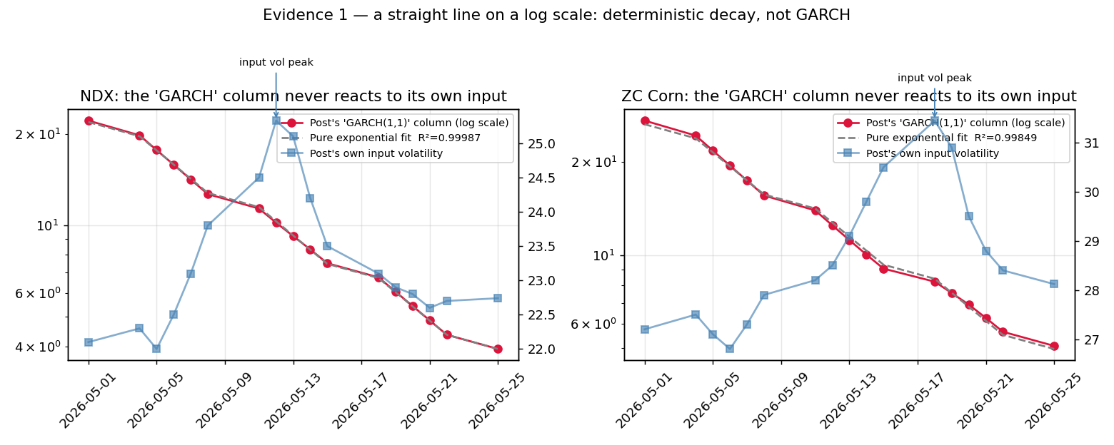
Cause: the variance recursion was iterated without its shock term
Whatever generated the table ran the decay part of the recursion and skipped the part that reads data. Two side findings confirm the column never touched reality: the “variance” column is initialized at the volatility level (22.10, 27.20) instead of vol² — a unit error — and the table contains a row for 2026-05-25, which was Memorial Day. US equities and the CME were closed; that trading day does not exist in real data (May 2026 had 16 sessions). The post was, fittingly, published on that same nonexistent trading day.
Effect 1: the column moves against its own input
A real conditional-volatility series co-moves with the volatility it conditions on. The post’s columns correlate at −0.269 (NDX) and −0.687 (ZC) with their own inputs — the “output” falls while its input spikes.
Effect 2: everything downstream inherits the defect
Regime labels, lag correlations, the hedging signal — every number computed from those columns is built on a series that contains no market information. The real refit over the same window behaves the way GARCH must: NDX conditional volatility (annualized %) oscillates 17.5 → 21.0 → 18.3, and ZC rises 16.9 → 28.4 in response to the grain shock.
The one-line takeaway
A GARCH series that never rises is not a GARCH series. Heteroskedasticity is the entire point.
Evidence 2: Why Is a Perfectly Symmetric Lead-Lag Correlation a Red Flag?
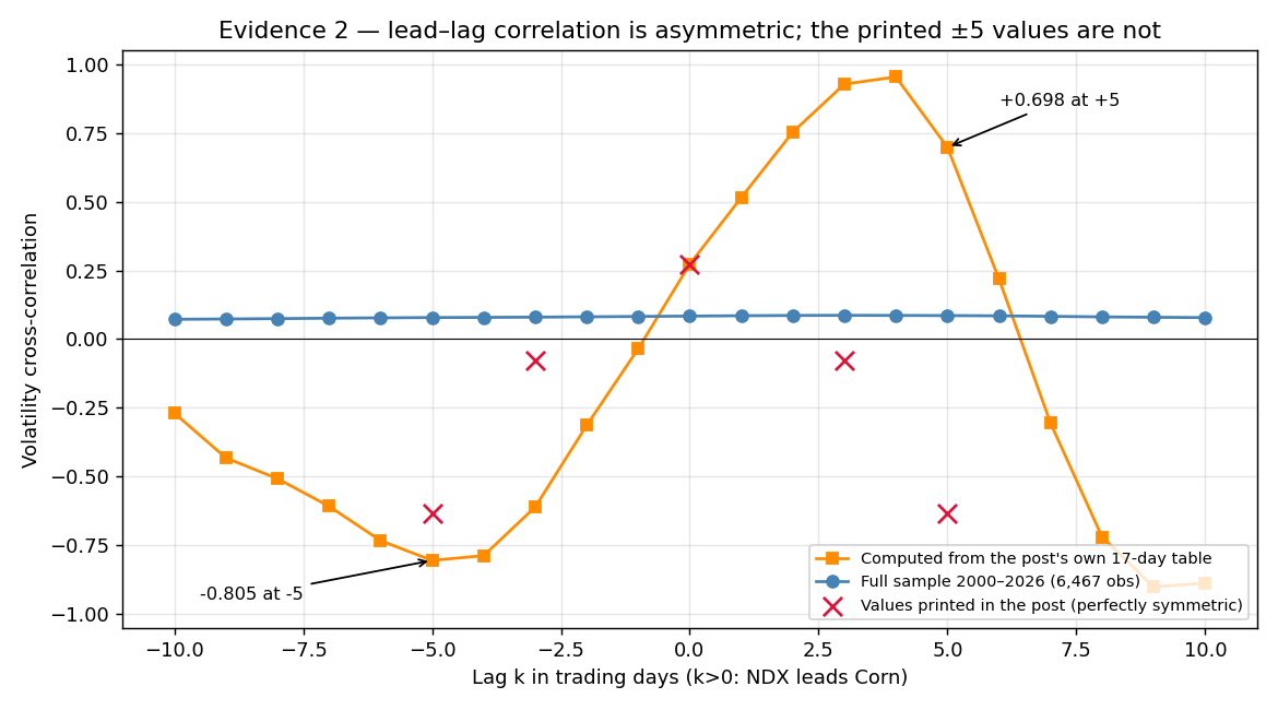
The original post printed the identical value at both lag +5 and lag −5: −0.6355 on each side. Call this the Mirror Artifact, because lead-lag correlation is asymmetric by construction:
$$\rho_{xy}(k) = \mathrm{corr}(x_{t-k},, y_t) ;\neq; \rho_{xy}(-k) \quad \text{in general}$$
At $+k$ and $-k$ you are correlating different pairs of observations — past-x-against-present-y versus future-x-against-present-y. Only degenerate special cases produce a mirror image, and a 17-row window of two distinct volatility series is not one of them.
So we recomputed the lead-lag correlations from the original post’s own printed 17-row table. The actual values:
| lag −5 | lag +5 | |
|---|---|---|
| Recomputed from the post’s own table | −0.805 | +0.698 |
| What the post printed | −0.6355 | −0.6355 |
Two independent failures in one number. First, the printed −0.6355 is not reproducible even from the post’s own table — the genuine computation gives +0.698 on one side and −0.805 on the other, strongly asymmetric and opposite in sign. Second, the exact ±5 symmetry is a shape that measured data does not produce. Whatever process printed that pair of numbers, it was not the correlation of those two columns. The ±3 pair shows the same mirror artifact — the post printed −0.0777 at both +3 and −3 — and while the printed lag-0 value of +0.2728 does reproduce from the post’s own 17-row table (+0.273), it diverges from the full-sample +0.084.
The one-line takeaway
If a lead-lag table is symmetric to four decimal places, the table is inconsistent with measured data. Recompute it from the raw columns before believing it.
Evidence 3: How Often Does a 17-Day Window Produce −0.6355 by Pure Chance?
Even setting both defects aside — suppose a 17-day window really had shown a large negative lag-5 correlation. Would that mean anything? This is where the full sample delivers the cleanest negative result of the audit.
Full-sample cross-correlation (real GARCH conditional volatilities, NDX leading at $k>0$, N = 6,467):
| $k$ | −10 | −5 | −3 | 0 | +3 | +5 | +10 |
|---|---|---|---|---|---|---|---|
| Real data | +0.072 | +0.079 | +0.080 | +0.084 | +0.087 | +0.086 | +0.078 |
| Original post’s claim | −0.6355 | −0.0777 | +0.2728 | −0.0777 | −0.6355 |
Flat. Between +0.07 and +0.09 at every lag from −10 to +10. No negative trough at lag 5, no trough anywhere. The DCC estimates agree:
- Lag 0: $a = 0.0032$, $b = 0.9938$ — a valid fit, with daily $\rho_t$ averaging +0.06 (std 0.04). The 5th-to-95th percentile band is +0.006 to +0.146: even the bottom tail stays positive.
- Lag 5: the shock parameter hits the $a = 0$ boundary, and the model degenerates to constant conditional correlation (CCC) with constant $\rho \approx 0.001$. There is no time-varying lag-5 correlation structure to estimate. The data declined to provide one.
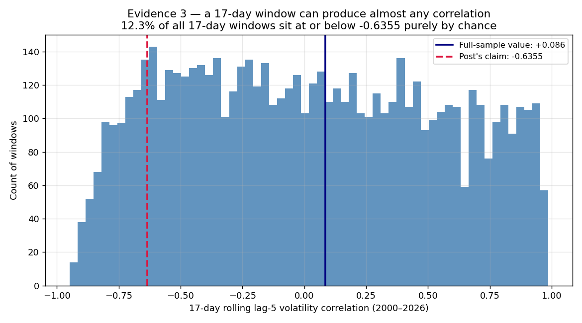
Now the small-sample punchline. We rolled the same 17-day lag-5 correlation the original post used across all 6,467 days. The rolling values swing from −0.95 to +0.99 — nearly the full mathematical range — and 12.3% of all windows reach ≤ −0.6355 by chance alone, in a population whose true cross-correlation is +0.08.
The arithmetic was always against a 17-day window: the Fisher standard error of a correlation at $N = 17$ is $1/\sqrt{N-3} \approx 0.267$ even for independent observations — and volatility series are nowhere near independent. With DCC persistence at $b = 0.9938$, adjacent days are almost copies of each other, so 17 rows hold far fewer than 17 effective observations. The 12.3% figure is the empirical measurement of that; the SE is the arithmetic intuition, not the proof.
The one-line takeaway
One in eight 17-day windows “discovers” a correlation this extreme in data where no such relationship exists. A 17-day correlation is not evidence. It is a lottery ticket.
What Is the Verdict?
This is a negative result, and we state it as one — what the data supports, and what fails:
| Claim | What the original post stated | Verdict | Key evidence |
|---|---|---|---|
| C1 — 5-day lagged negative transmission | NDX→ZC volatility reaches maximum negative correlation (r = −0.6355) at a 5-business-day lag | Refuted | Full-sample cross-correlation is flat at +0.07 to +0.09 across all lags ±10; lag-5 DCC degenerates to constant $\rho \approx 0.001$; −0.6355 is not reproducible even from the post’s own table |
| C2 — three volatility regimes with distinct relationships | K-Means splits the market into 3 regimes; the NDX–ZC relationship differs by regime | Partially confirmed | 3-regime separation holds and is statistically significant (Kruskal-Wallis p ≈ 2×10⁻²⁹), but the effect size is Δρ ≈ 0.02 with invariant sign (+0.05 to +0.08 in every regime) — economically meaningless |
| C3 — the table’s GARCH(1,1) estimates match a real fit | Published conditional-volatility columns are genuine GARCH output | Refuted | Columns are pure exponential decay ($R^2 > 0.998$), no shock response, negative correlation with their own inputs — a pipeline error, inconsistent with the real refit |
On C2, the three regimes themselves separate cleanly — R0 grain-volatility expansion (n = 1,688), R1 calm (n = 4,016), R2 equity stress (n = 763) — but note the trap in miniature: at N ≈ 6,400, a p-value of 2×10⁻²⁹ will flag differences far too small to trade. Statistical separation is real; an actionable regime relationship is not. Statistically significant ≠ economically meaningful — the sign of the NDX–ZC correlation never changes across regimes.
What survives, for the record: the VXN level of 25.33 was the genuine May 2026 high — but the real VXN recorded it on May 15, not the May 12 the post printed (the post’s NDX_Vol column correlates +0.707 with real VXN, mean absolute error 0.62pt — derived from reality, but not equal to it). The Sharpe improvement claim (1.15 → 1.84) is withdrawn outright: with no lag structure, there is no premise to compute it from. And the post’s DTW framing is withdrawn with it — no reproducible computation behind it was found. Withdrawn as well: one quotation whose source could not be externally verified.
What Do We Take Away From Auditing Ourselves?
Lesson 1: small-sample correlations are lottery tickets, and persistence makes them worse
Every danger in this audit compounds in small windows. The Fisher SE says $\pm 0.27$ at N = 17; persistence (b = 0.9938) shrinks the effective sample further; and the empirical exceedance — 12.3% of windows at or below the headline value — is the measured price of trusting one window. If your headline number comes from fewer than 30 observations of a persistent series, roll the same window across all the history you have and report the chance-alone exceedance rate next to it. If you can’t survive publishing that rate, don’t publish the number.
Lesson 2: GARCH outputs can be audited in five lines — so audit them
Every red flag in our own table was machine-detectable. The pitfall table:
| Defect | Symptom | Remedy |
|---|---|---|
| Shock-blind variance recursion | Conditional-vol column decreases monotonically through input spikes | Require corr(output, input) > 0; verify the column rises within 1–2 steps of an input spike |
| Pure exponential decay | Log-linear fit with $R^2 > 0.99$, constant per-step factor | Regress $\log \sigma_t$ on $t$; an almost-perfect line means the data was never read |
| Mirror-symmetric lead-lag table | Identical correlation printed at $+k$ and $-k$ | Recompute $\rho(\pm k)$ from the raw columns; expect asymmetry |
| Small-sample correlation | |r| > 0.6 at N < 30 | Roll the same window across the full sample and report the chance-alone exceedance rate |
| Variance/volatility unit mix-up | “Variance” column initialized at the volatility level | Confirm variance ≈ vol²; hand-check one row |
| Calendar contamination | Rows on exchange holidays (e.g., 2026-05-25, Memorial Day) | Validate every date against the exchange trading calendar |
| Non-reproducible N | Sample size exceeds what the named data source can supply | Recount the sample from the raw download before quoting N |
Here is the corrected implementation — the exact forensic check that closed C3, plus the two-liner behind the 12.3% figure:
import numpy as np
import pandas as pd

def audit_garch_column(garch_col: pd.Series, input_vol: pd.Series) -> dict:
    """Forensic audit for a column claiming to be GARCH(1,1) conditional volatility.

    On the original post's NDX column this returned:
    monotone_decay=True, loglinear_r2=0.99987, corr_with_own_input=-0.269
    -> verdict: pipeline error, not a GARCH output.
    """
    out = {}

    # Red flag 1 — monotone decay: real GARCH must rise after shocks
    # because of the alpha * eps^2 term in sigma^2_t.
    out["monotone_decay"] = bool((garch_col.diff().dropna() < 0).all())

    # Red flag 2 — log-linear fit: pure exponential decay gives R^2 ~ 1.
    y, t = np.log(garch_col.to_numpy()), np.arange(len(garch_col))
    slope, intercept = np.polyfit(t, y, 1)
    resid = y - (slope * t + intercept)
    out["loglinear_r2"] = float(1 - resid.var() / y.var())
    out["decay_factor_per_step"] = float(np.exp(slope))

    # Red flag 3 — shock response: conditional vol must co-move with its input.
    out["corr_with_own_input"] = float(garch_col.corr(input_vol))

    failed = (out["monotone_decay"]
              and out["loglinear_r2"] > 0.99
              and out["corr_with_own_input"] <= 0)
    out["verdict"] = "pipeline error - not a GARCH output" if failed \
                     else "passes basic GARCH sanity checks"
    return out

# The 12.3% measurement: roll the post's own 17-day lag-5 window
# across all 6,467 days and count chance-alone exceedances.
roll_corr = vol_ndx.shift(5).rolling(17).corr(vol_zc).dropna()
print(f"{(roll_corr <= -0.6355).mean():.1%}")   # 12.3%
Lesson 3: a negative result that closes a question beats a positive result that opens one
The most useful output of this audit is the flat line: +0.07 to +0.09 at every lag, lag-5 DCC degenerate at $a = 0$. That is a completed conclusion. Nobody reading this needs to wonder whether a cleverer window or a different lag rescues the corn hedge — the full sample answered, and the answer is no. The corrected original post now says exactly that, and the two posts cross-reference so neither version of the record can circulate without the other.
The uncomfortable part of publishing an autopsy of your own work is also the entire value of it: the audit trail is now public, the red-flag checks are now code, and the same checks are being run against our other published tables.
The most dangerous backtest to audit is the one you already published. Audit it anyway — before a reader does it for you.
Run the three red-flag checks above against your own published numbers this week. If a column fails, write the correction notice the same day. The numbers were always going to be re-checked by someone; the only choice you control is whether your name is on the audit.
FAQ: Self-Audits, Negative Results, and GARCH Forensics
What exactly is DCC-GARCH, and why was it the right tool for this re-validation?
DCC (Dynamic Conditional Correlation) GARCH, introduced by Engle (2002), is a two-stage model: stage one fits univariate GARCH(1,1) to each return series and extracts standardized residuals; stage two estimates a time-varying correlation $\rho_t$ between them, governed by shock and persistence parameters $a$ and $b$. It was the right tool because the original claim was about a correlation structure — and DCC tests whether that structure exists dynamically rather than reading one static Pearson number off a 17-row window. On the lag-5 pair, the fit returned $a = 0$, degenerating to constant correlation ≈ 0.001: no structure.
Why publish a full self-audit instead of quietly editing the original post?
Because the original numbers were public for seventeen days, and a quiet edit leaves every cached copy, screenshot, and reader memory uncorrected with no way to discover the change. A public negative result does three jobs at once: it closes the empirical question (the structure does not exist in 6,467 days of data), it documents how the defect arose (a pipeline error, with the forensic evidence preserved), and it hands readers the exact checks — monotone decay, mirror symmetry, small-sample exceedance — to audit anything else we publish.
What survived the audit of the original post?
Three things. The VXN level of 25.33 was the genuine May 2026 high — recorded on May 15, not the May 12 the post printed. The 3-regime K-Means classification (C2) separates with Kruskal-Wallis p ≈ 2×10⁻²⁹ — though with Δρ ≈ 0.02 and an invariant positive sign it carries no economic content. And the GARCH(1,1)/K-Means methodology itself remains valid; what failed was the output presented as coming from it. Refuted: the 5-day-lag negative correlation (C1) and the published GARCH table (C3), plus everything built on them — the hedging timing rule, the Sharpe improvement claim, and the DTW framing.
What does the 12.3% figure actually mean?
It is the measured chance-alone exceedance rate. Rolling the original’s own 17-day lag-5 window across all 6,467 trading days, 12.3% of windows reached the original’s −0.6355 level or below in data whose true full-sample correlation is +0.08. Two compounding effects make that possible: arithmetically, the standard error of a correlation at N = 17 is about $1/\sqrt{14} \approx 0.27$, so extreme values are only ~2.4 standard errors out even under independence; empirically, volatility series are highly persistent (our DCC fit shows $b = 0.9938$), so consecutive days are nearly duplicates and the effective sample is far smaller than 17.
Why is a monotonically decreasing GARCH column a definitive red flag rather than a borderline one?
Because the GARCH(1,1) recursion $\sigma_t^2 = \omega + \alpha\varepsilon_{t-1}^2 + \beta\sigma_{t-1}^2$ guarantees that conditional variance rises after a large shock whenever $\alpha > 0$ — and an estimated $\alpha$ of zero on real financial data would itself be a fit failure. Seventeen consecutive decreases through two separate input volatility peaks is not a borderline pattern; combined with a log-linear $R^2$ of 0.99987, it identifies the column as a deterministic decay that never read the data.
Related Research
- The complete picture — start with the hub: 7 Ways Your Backtest Is Lying to You (Measured, Not Guessed) — the pipeline error and the small-sample lottery this audit forensically documented are two of the seven; the hub indexes the remaining five, each wired to its own full experiment.
- The post under audit: Is Buying Corn Futures Safe When Stocks Crash? — the corrected original, now reflecting the full-sample results documented here.
- The Backtest Autopsy Series:
- The Backtest Autopsy #1: Entry Price is the Edge: This audit traced how one mis-fed variance column silently corrupted every downstream number; Autopsy #1 traces the same kind of compounding distortion back to the entry-price assumption instead.
- Debugging the Look-Ahead Bias ChatGPT Can Never Catch: The look-ahead checklist item we ran and passed in Phase 2 above is a single line item; this piece turns that same discipline into a full protocol for catching leaked future data before it ever reaches a claim.
- Slippage Simulation: Measuring Execution Latency and Account Decay: Where this audit reconciled a printed correlation table against the real GARCH math, this piece reconciles paper-backtest fills against what a live order actually pays to get filled.
- Why Your Backtest Changes When You Switch Timeframes: The 12.3% chance-alone exceedance rate above and this piece’s 50:50 coin-flip result are the same species of finding — a number that reads like an edge until you measure how often chance alone produces it.
- Correlation is Not Directional: Statistically Demystifying Multi-Asset Convergence: The flat +0.07 to +0.09 cross-correlation this audit measured is a live example of exactly the trap this piece formalizes — a correlation that is real and still implies no tradeable direction.
Last verified: June 2026
Sources & data: Yahoo Finance daily closes via
yfinance(^NDX 1985–2026, ZC=F 2000–2026, ^VXN May 2026); GARCH(1,1) and two-stage DCC(1,1) estimation in Python (reference implementation pre-validated on synthetic data with known parameters); K-Means clustering via scikit-learn KMeans++; model background: Autoregressive conditional heteroskedasticity — Wikipedia; Engle, R. F. (2002), Dynamic Conditional Correlation, Journal of Business & Economic Statistics 20(3).
Key figures
Frequently asked
What is a DCC-GARCH model and what does it measure?
Why publish a negative result instead of quietly fixing the post?
What survived the audit of the original post?
What does the 12.3% figure mean?
Why is a monotonically decaying GARCH column a red flag?
Sources
- Autoregressive Conditional Heteroskedasticity (ARCH/GARCH) — Wikipediaen.wikipedia.org
- scikit-learn — sklearn.cluster.KMeans (k-means++ initialization)scikit-learn.org
- Engle, R. F. (2002). Dynamic Conditional Correlation — A Simple Class of Multivariate GARCH Models. Journal of Business & Economic Statistics, 20(3)
Educational content only — not investment or financial advice. Data, prices, and tool specifications change; verify independently and paper-trade before risking capital.