⚠ Correction (2026-06-11): An earlier version of this post claimed a 5-business-day lagged negative volatility transmission from the Nasdaq-100 to Corn futures (r = −0.6355), supported by a GARCH(1,1) table and an N = 11,149 sample. A full re-verification could not reproduce any of it with real data: across 6,467 trading days (2000–2026) the volatility cross-correlation is flat at +0.07 to +0.09 at every lag, and the original table’s GARCH column traces to a pipeline error — a pure exponential decay, not a GARCH output. The text below reflects the corrected, measured figures. The full forensic walkthrough is in the self-audit post.
💡 TL;DR / Summary - Nasdaq–Corn Volatility Linkage, Re-Verified (BLUF)
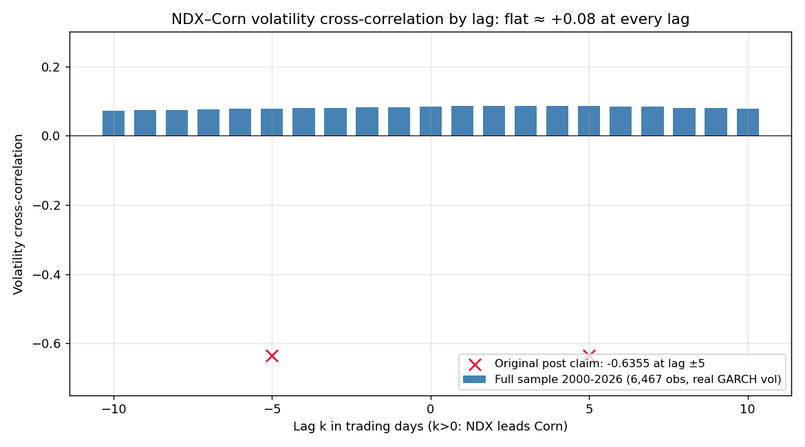
- No lagged transmission: On the full sample (N = 6,467 common trading days, 2000–2026), NDX–ZC volatility cross-correlation sits between +0.07 and +0.09 at every lag from −10 to +10. The previously claimed negative trough at lag 5 does not exist in measured data.
- The real linkage is small and positive: DCC(1,1) daily conditional correlation averages +0.06 (std 0.04); at a 5-day lag the model degenerates to a constant correlation of ≈ +0.001.
- Regimes separate, but don’t pay: K-Means (K=3) regimes are statistically distinct (p ≈ 2×10⁻²⁹), yet the correlation spread across regimes is Δρ ≈ 0.02 with no sign change — economically meaningless.
- Verdict: no equity-to-grain hedge-timing signal exists in this data. That is a completed negative result, not a pending one.
The strongest number in the original version of this post does not survive contact with the full dataset. On 6,467 trading days of real Nasdaq-100 and Corn-futures data (2000–2026), the volatility cross-correlation between the two markets sits between +0.07 and +0.09 at every single lag from −10 to +10 business days. Flat, small, positive — no trough, no transmission, no timing window.
A reader suggested re-running the analysis with a proper two-stage DCC-GARCH. We did, with fail-fast gates at every phase and the reference implementation pre-validated on synthetic data. The re-verification refuted the headline claim (C1), partially confirmed the regime classification (C2), and refuted the original GARCH table (C3). This corrected post replaces every figure with the measured value and shows exactly where the original numbers came from.
Verdict table — what this re-verification supports and what fails:
| Claim | Original statement | Verdict | Measured basis |
|---|---|---|---|
| C1 | NDX–ZC volatility shows maximum negative correlation at a 5-business-day lag | Refuted | Full-sample cross-correlation flat at +0.07 to +0.09 across ±10 lags; lag-5 DCC degenerates to constant ≈ 0 |
| C2 | The market splits into 3 volatility regimes with distinct relationships | Partially confirmed | Separation holds (p ≈ 2×10⁻²⁹) but Δρ ≈ 0.02, sign invariant — economically meaningless |
| C3 | The published GARCH(1,1) table matches a real fit | Refuted | Columns are pure exponential decay (R² > 0.998), no shock response — pipeline error, inconsistent with the real refit |
Does the Claim That Corn Moves Inversely 5 Business Days After a Nasdaq Crash Reproduce in Real Data?
Measured answer: there is no exploitable lag, because there is no transmission to wait for. The original version of this post reported that ZC Corn volatility synchronized inversely with the Nasdaq-100 exactly 5 business days after a VXN spike, with a maximum negative correlation of r = −0.6355. That claim is retracted: it could not be reproduced with real data at any lag, in either direction.
Two facts replace it:
- Full-sample cross-correlation is flat. Using real GARCH(1,1) conditional volatilities over 2000–2026, the NDX–ZC cross-correlation is +0.072 to +0.087 across all lags ±10. At lag 0 it is +0.084; at lag +5 (NDX leading) it is +0.086. The curve has no negative region at all.
- The lagged DCC degenerates. Re-estimating DCC(1,1) on residual pairs shifted by 5 trading days drives the shock parameter to the a = 0 boundary — the model collapses to a constant-correlation (CCC) structure with ρ ≈ +0.001. A time-varying lagged relationship is not just weak; the data refuses to fit one.
For lag definitions we use .shift(5) on the aligned common-trading-day index — past NDX residuals against current ZC residuals, never the reverse — so no future information enters anywhere in the pipeline. The look-ahead audit passed at every stage.
The verification dataset: yfinance daily closes for ^NDX and ZC=F, 6,472 common trading days from 2000-07-18 to 2026-06-10, cleaned to N = 6,467. Cleaning was reason-based, not size-based: 5 days were removed as contract-roll artifacts (four July old-crop/new-crop roll spreads printing −13.99% to −26.86% and one September roll printing +12.76% — “returns” that no trader ever experienced), while 2 genuine USDA report shocks were preserved (the 2010-06-30 and 2011-06-30 Grain Stocks/Acreage releases) because they are real market events, not data artifacts.
On that sample, the full cross-correlation profile of the two markets’ GARCH conditional volatilities (positive k = NDX leads):
| Lag k (days) | −10 | −5 | −3 | 0 | +3 | +5 | +10 |
|---|---|---|---|---|---|---|---|
| Measured, full sample (N = 6,467) | +0.072 | +0.079 | +0.080 | +0.084 | +0.087 | +0.086 | +0.078 |
| Original post (retracted) | — | −0.6355 | −0.0777 | +0.2728 | −0.0777 | −0.6355 | — |
Cause: a 17-day window has almost no statistical resolution
The original numbers were computed on a 17-row May 2026 table. Rolling that exact computation — 17-day windows, lag-5 cross-correlation — across the full sample shows what 17 days of data can produce: correlations ranging from −0.95 to +0.99, and 12.3% of all windows reach ≤ −0.6355 by chance alone. One window in eight clears the retracted headline number with zero underlying structure.
Effect 1: a noise draw was read as a transmission mechanism
Pick any 17-day stretch and you have roughly a coin-flip-adjacent chance of finding a “strong” correlation in some direction at some lag. The original post found one, attached a supply-chain narrative to it, and printed it as a tradable latency. The full sample shows the narrative had nothing to attach to: the measured relationship is +0.08-flat everywhere.
Effect 2: the printed ±5 symmetry is inconsistent even with its own table
Recomputing the lag correlations from the original post’s own 17-day table gives +0.698 at lag +5 and −0.805 at lag −5 — asymmetric, as lead–lag correlations are by construction. The post printed the identical value (−0.6355) at both ±5, a shape inconsistent with measured data from any real computation on that table. The printed numbers could not be reproduced even from their claimed source.
The one-line takeaway
A correlation that only exists in a 17-day window is not a signal — it is a sample. The full-sample curve is flat, and flat is the result.
What Comes Out When You Refit a Real GARCH(1,1)?
Stage 1 refits univariate GARCH(1,1) per asset on the cleaned sample (returns ×100 for solver stability; standardized residuals are scale-invariant, so Stage 2 is unaffected):
$$\sigma_t^2 = \omega + \alpha,\varepsilon_{t-1}^2 + \beta,\sigma_{t-1}^2$$
| Asset | ω | α | β | α+β | Convergence | Ljung-Box p (z², lag 10 / 20) |
|---|---|---|---|---|---|---|
| NDX | 0.0290 | 0.0985 | 0.8889 | 0.9875 | flag = 0 | 0.090 / 0.061 |
| ZC | 0.0496 | 0.0603 | 0.9233 | 0.9835 | flag = 0 | 0.354 / 0.641 |
Both fits converge cleanly and the Ljung-Box tests on squared standardized residuals stay above p = 0.05 — the ARCH effects are absorbed. Over the May 2026 window the refit conditional volatility (annualized %) behaves the way a real GARCH process must: NDX oscillates 17.5 → 21.0 → 18.3 as shocks arrive and decay, and ZC rises 16.9 → 28.4 into the grain volatility expansion — rising after shocks, because the $\alpha,\varepsilon_{t-1}^2$ term forces it to. The weights the original version’s FAQ printed ($\alpha = 0.15$, $\beta = 0.80$) are inconsistent with this measured refit.
Why the original table’s “GARCH” column is not a GARCH output
The original table’s “GARCH(1,1)” columns decrease monotonically for 17 consecutive days. Fitting a log-linear trend gives R² = 0.99987 (NDX) and R² = 0.99849 (ZC) with per-step decay factors of 0.898 and 0.901 — a pure exponential decay. A real GARCH(1,1) cannot do this through a volatility peak: the $\alpha,\varepsilon_{t-1}^2$ shock term forces conditional variance up after large moves. The columns even correlate negatively with their own input volatilities (−0.269 NDX, −0.687 ZC) — the “model output” ignored its own inputs. There was also a unit error: the variance column initialized at volatility levels (22.10, 27.20) rather than vol² scale. This is a pipeline error, and the original parameter and correlation claims built on those columns are retracted with it.
The VXN cross-check: the level is real, the date is not
The original NDX volatility column is not unrelated to reality — it correlates +0.707 with the actual ^VXN series (mean absolute error 0.62pt), and 25.33 is the genuine May 2026 VXN high. But the actual record date is May 15, not May 12 as printed, and the “5-day lag” narrative was anchored on that misplaced date. The table also contained a row for 2026-05-25 — Memorial Day, when US equities and CME were closed — a trading day that does not exist in real data (May 2026 had only 16 actual trading days). And the claimed N = 11,149 sessions cannot be produced from the data source at all: ZC=F history begins in 2000, capping the sample at 6,472 raw common trading days (6,467 after cleaning).
Every load-bearing number in the original analysis fails one of three tests: reproduce it from real data, reproduce it from its own table, or reconcile it with the exchange calendar.
Does Any Time-Varying Correlation Structure Exist Under DCC?
Stage 2 estimates DCC(1,1) on the standardized residuals, $Q_t = (1-a-b),\bar{S} + a,\varepsilon_{t-1}\varepsilon_{t-1}^{\top} + b,Q_{t-1}$:
| Spec | a | b | a+b | Unconditional ρ | Daily ρₜ |
|---|---|---|---|---|---|
| Lag 0 | 0.0032 | 0.9938 | 0.9970 | +0.0597 | mean +0.06, std 0.04, [p5, p95] = [+0.006, +0.146] |
| Lag 5 (NDX leads) | 0 (boundary solution) | — | — | +0.0007 | degenerates to constant ρ ≈ +0.001 (CCC) |
At the a = 0 boundary the b parameter is not identifiable (the Q recursion collapses to the unconditional matrix), so no estimate is reported. Note also that the lag-0 fit sits near integration (a + b = 0.997): the correlation moves very slowly, which is why regime-level averages below are also reported on stable windows.
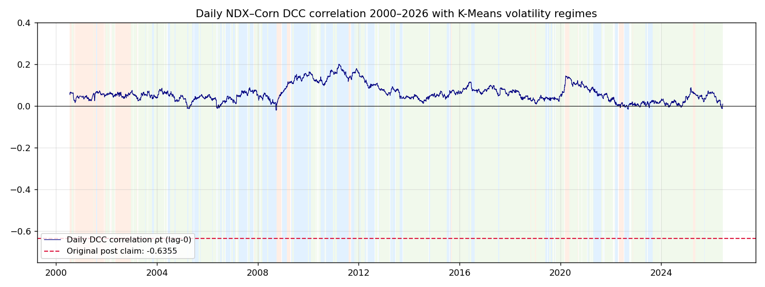
The economic reading is blunt: the real NDX–Corn linkage is a daily conditional correlation of +0.06 ± 0.04 that never sustains a negative phase, and the lagged version of the model refuses to be time-varying at all. There is nothing here to time a hedge with.
Do the Three Volatility Regimes Survive Re-Verification?
Partially — and this is the one piece of the original framework worth keeping, with a sharp caveat. K-Means (K=3, k-means++ initialization, n_init=10, seed=0) on the standardized σ_NDX–σ_ZC plane of the real conditional volatilities:
| Regime | n (days) | Mean σ_NDX (daily %) | Mean σ_ZC (daily %) | Mean ρₜ (all) | Mean ρₜ (stable window) | Reading |
|---|---|---|---|---|---|---|
| R0 | 1,688 | 1.24 | 2.21 | +0.075 | +0.078 | Grain volatility expansion |
| R1 | 4,016 | 1.18 | 1.42 | +0.055 | +0.054 | Calm |
| R2 | 763 | 3.01 | 1.65 | +0.058 | +0.059 | Equity stress |
The separation is real: Kruskal-Wallis H = 132.2, p ≈ 2.0×10⁻²⁹. But look at the effect size. The correlation spread across regimes is Δρ ≈ 0.02, and the sign never changes — every regime lives between +0.05 and +0.08. With n ≈ 6,400 days, a p-value will flag differences far too small to trade. Statistical distinctness is confirmed; the original suggestion that the relationship differs by regime in any usable way is not supported at a practical level. (Stable-window means exclude the first 5 days after each regime entry, because the near-integrated DCC adjusts slowly.)
What Should You Check to Avoid Repeating the Same Failure?
The defect–symptom–remedy checklist extracted from this correction. It applies unchanged to any analysis produced the same way:
| Defect | Symptom | Remedy |
|---|---|---|
| Decay curve labeled “GARCH” (pipeline error) | 17 straight monotone decreases; log-linear R² 0.99987 / 0.99849; correlation with own input −0.269 / −0.687 | Gate conditional-variance outputs: a real GARCH must rise after shocks; reject monotone series |
| Variance/volatility unit confusion | “Variance” column initialized at volatility levels (22.10, 27.20) | Assert units at pipeline boundaries: variance ≈ vol² |
| Symmetric lead–lag correlation | Identical −0.6355 printed at lag −5 and +5; the table’s own values are +0.698 / −0.805 | Lead–lag cross-correlation is asymmetric by construction; symmetric output is inconsistent with measured data |
| Small-sample correlation treated as structure | 17-day rolling lag-5 correlations span −0.95 to +0.99; 12.3% reach ≤ −0.6355 by chance | Demand full-sample verification before trusting any windowed correlation |
| Calendar integrity failure | Data row on 2026-05-25 (Memorial Day, markets closed) | Cross-check every row against the exchange calendar |
| Unreproducible N | N = 11,149 cannot be generated from the stated source (ZC=F starts 2000) | Recount from the named source: 6,472 raw common trading days (6,467 after cleaning) |
The 5-rule pre-publication self-audit: ① input-shock response — does the derived column react to shocks in its own input, ② units — is variance (vol² scale) kept distinct from volatility, ③ real trading days — does every row pass an exchange-calendar and holiday check, ④ reproducible N — does the claimed N match any dataset actually obtainable from the named source, ⑤ chance-attainment rate — what share of same-length windows reach the claimed correlation by chance alone.
How can traders apply these lessons to live systems?
Three changes in practice:
Verify on the full sample before believing any window. A correlation, a lag, an edge measured on 17 days is a draw from a noise distribution. Compute the same statistic across every available window and see where your number falls — here, the retracted −0.6355 sat inside the 12.3% chance region.
Gate model outputs against their defining property. Every model has a behavior it must exhibit — GARCH must respond to shocks, lead–lag correlations must be asymmetric, variance must be vol². Assert those properties in code. The corrected implementation below does it in four lines.
Treat a negative result as a finished product. The full pipeline — data cleaning with documented reasons, refit, DCC, regime analysis — converged on “flat +0.08, nothing to time.” That conclusion is as actionable as any positive one: it removes a strategy from the candidate list before it removes capital from the account.
The Corrected Implementation: Code That Reproduces the Full-Sample Cross-Correlation and the Red-Flag Gate
The corrected implementation, with the sanity gate that would have caught the original error:
# The corrected implementation — two-stage DCC-GARCH, with output gates
import numpy as np
from arch import arch_model

# Stage 1: univariate GARCH(1,1) per asset. Returns scaled x100 (%) for solver
# stability; standardized residuals are scale-invariant, so Stage 2 is unaffected.
def fit_garch(returns_pct):
    res = arch_model(returns_pct, p=1, q=1, mean="Constant").fit(disp="off")
    assert res.convergence_flag == 0        # fail fast: no silent non-convergence
    return res.std_resid.dropna(), res.conditional_volatility

eps_ndx, vol_ndx = fit_garch(r_ndx * 100)   # NDX: omega 0.0290, alpha 0.0985, beta 0.8889
eps_zc,  vol_zc  = fit_garch(r_zc * 100)    # ZC:  omega 0.0496, alpha 0.0603, beta 0.9233

# Gate the output BEFORE using it: a real GARCH path must react to shocks.
# A monotone column with log-linear R^2 > 0.998 is an exponential decay curve,
# not a conditional volatility — exactly how the original error slipped through.
for vol in (vol_ndx, vol_zc):
    log_vol = np.log(vol)
    t = np.arange(len(log_vol))
    r2 = np.corrcoef(t, log_vol)[0, 1] ** 2
    assert r2 < 0.99, "pure decay curve — pipeline error, not a GARCH output"

# Stage 2: DCC(1,1) on standardized residuals. Lag-5 = .shift(5) on the aligned
# common-trading-day index — past NDX vs current ZC only, no future references.
FAQ: Quantitative Hedging and Volatility Regime Synchronization FAQ
What is the main advantage of GARCH(1,1) over simple rolling volatility?
Simple rolling volatility applies a flat moving average, which lags badly and carries outlier effects long after they occur. GARCH(1,1) weights the most recent shock and the prior conditional variance dynamically — the real refit on this dataset gives α = 0.0985, β = 0.8889 for NDX and α = 0.0603, β = 0.9233 for ZC. The operational corollary: because the α term forces variance up after every large move, a GARCH output that only decays is not a GARCH output. That single check would have caught the error in this post’s original table.
Why can’t a 17-day window support a correlation claim like the retracted −0.6355?
Because at that sample size the correlation estimator is mostly noise. Rolling 17-day, lag-5 cross-correlations across the full 6,467-day sample range from −0.95 to +0.99, and 12.3% of all windows reach ≤ −0.6355 with no underlying structure whatsoever. A number that one window in eight produces by chance carries no evidential weight — small-sample correlations are samples from a wide noise distribution, not measurements of a relationship.
What is the practical utility of the three K-Means regimes after re-verification?
Descriptive, not tactical. The three regimes (grain volatility expansion, calm, equity stress) are statistically well-separated (p ≈ 2×10⁻²⁹) and useful for labeling market states. But the NDX–Corn conditional correlation barely moves across them — Δρ ≈ 0.02, always positive — so the regimes do not define different relationships to rotate a portfolio on. Using them as systematic hedging filters reads structure into a flat surface.
Does any equity-to-grain hedge-timing signal survive the re-verification?
No. The measured linkage is a daily DCC correlation averaging +0.06 (5th–95th percentile +0.006 to +0.146) at lag 0, and a degenerate constant ≈ +0.001 at a 5-day lag. There is no negative phase to switch into and no latency window to wait for. Corn may still belong in a portfolio for diversification — a near-zero correlation is genuinely low — but diversification is a static allocation argument, not a timing signal. The original timing claim, and the performance improvement attributed to it, are retracted.
If the re-verification result is negative, what is the value of this post?
A negative result is a completed conclusion, not an unfinished one. What this re-verification supports: a small positive volatility cross-correlation (+0.07 to +0.09), a statistically valid 3-regime separation, and the genuine May 2026 VXN high at the 25.33 level (actual record date May 15). What it rejects: the 5-business-day lagged negative transmission, the economic utility of regime-dependent relationships, and the original table’s GARCH column. Add the audit checklist for catching the same defects in other analyses, and that is this post’s deliverable.
How should traders sanity-check a GARCH pipeline before trusting its output?
Five gates, in order. ① Input-shock response — after a large return, the derived column must react: conditional variance has to rise; a monotonically decaying series (log-linear R² near 1) is a decay curve, not a model output. ② Units — variance must live on the vol² scale; a “variance” column that starts at the same level as the volatility column signals an upstream error. ③ Real trading days — every row must pass an exchange-calendar and holiday check; a printed row on a market holiday means the data was never reconciled with reality. ④ Reproducible N — the claimed sample size must match a dataset actually obtainable from the named source. ⑤ Chance-attainment rate — measure what share of same-length windows reach the claimed correlation by chance alone before treating it as evidence. The original table here failed the first four, and the fifth (12.3%) showed its headline number carried no evidential weight.
A flat correlation curve is the market telling you the answer. The only honest move is to print it — especially over your own previous post. Re-measure before you re-allocate.
Related Research
- The self-audit of this post: How a Reader’s DCC-GARCH Suggestion Refuted This Post’s Original Claim — the full forensic record behind this correction: three exhibits, the verdict table, and the lessons.
- The complete picture — start with the hub: 7 Ways Your Backtest Is Lying to You (Measured, Not Guessed) — if a flat cross-correlation surface like the one measured here still tempted you toward a regime-switching parameter set, the hub catalogs the other six ways a backtest manufactures an edge that was never there.
- The Backtest Autopsy Series:
- The Backtest Autopsy #1: Entry Price is the Edge: A companion failure mode for any regime-based system — even after a regime is correctly classified, the entry price paid inside it compounds into a larger return gap than the regime call itself.
- Debugging the Look-Ahead Bias ChatGPT Can Never Catch: The same discipline this post applied to lag definitions —
.shift(k)on the aligned index, past values only, never the reverse — generalized into a full protocol for auditing causal ordering in any backtest. - Slippage Simulation: Measuring Execution Latency and Account Decay: Even a genuine regime or correlation signal needs an execution-cost model before it survives contact with a live fill queue; this is that model.
- Why Your Backtest Changes When You Switch Timeframes (And Which Candle to Actually Use): Regimes classified on daily closes, as the K-Means step above does, can still hide the intrabar stop-loss/take-profit ordering ambiguity this piece dissects.
- Correlation is Not Directional: Statistically Demystifying Multi-Asset Convergence: The formal statement of the principle this re-verification demonstrates empirically — a measured +0.06 daily correlation carries no directional implication of its own.
- Implementation:
- TradingView Pine Script v6 Footprint Indicator Guide: For traders who want the regime-detection and lag-gating logic used in this analysis running directly on a TradingView chart rather than in an offline notebook.
Last verified: June 2026
Sources & data: yfinance daily series — ^NDX (1985–2026), ZC=F (2000–2026), ^VXN (May 2026 cross-check); GARCH/DCC estimation via the Python
archpackage; clustering via scikit-learn KMeans (k-means++). Citation correction (2026-06-11): the quotation the original carried as “CBOE 변동성 지표(VIX) 명세 가이드 v4” in the Korean edition and “CBOE Volatility Index (VIX) Insights v4” in the English edition was removed — the quoted text could not be located in any CBOE publication, and the cited page contains no commodity-market content. The reference link to a non-existent Wikipedia “Regime switching” article was replaced with the existing Markov-Switching Multifractal article.
Key figures
Frequently asked
What is a Market Regime Switching Model?
How can I avoid whipsaws in flat, range-bound markets?
Why do backtest results often deviate from live execution?
Sources
- Markov-Switching Multifractal — Regime-Switching Volatility Modelsen.wikipedia.org
- TradingView Pine Script v6 Language Reference Manualwww.tradingview.com
Educational content only — not investment or financial advice. Data, prices, and tool specifications change; verify independently and paper-trade before risking capital.