💡 Bottom Line
- A crypto perpetual-futures backtest fails live for five reasons, but only two are crypto-specific: notional-based funding drag and silent data gaps. Fix those here.
- The other three (limit-fill illusion, slippage and latency, look-ahead bias via joins) are universal backtest sins that apply to stocks, FX, and futures alike. We measured each one with real data in the Backtest Autopsy series, so this guide links out instead of repeating them.
- The funding numbers below are worked calculations from stated assumptions, not a measured study. The measured forensics live in the linked spokes.
This is a methodology guide, not a forensic report. Where a claim needs measured proof, we point to the specific Backtest Autopsy spoke that measured it, rather than reproducing numbers here.
1. Why this guide exists
Most articles on “crypto backtest pitfalls” list ten generic mistakes that apply to any market and stop there. That framing obscures the only two problems that are truly unique to crypto perpetual futures: funding costs are charged on leveraged notional value, and 24/7 historical data must be stitched together from sources that silently drop bars.
Consequently, we have split the five graveyards into two categories. The two crypto-specific pitfalls receive in-depth analysis here, complete with a corrected funding formula and code implementation. The three universal traps each receive a concise summary paragraph with a link to the specific spoke that measured them. To maintain consistency, no empirical data is duplicated across this cluster.
2. Crypto graveyard #1: notional funding drag
The most costly mistake in perpetual-futures backtesting is treating the funding fee as a negligible percentage of account equity, or omitting it entirely.
Funding is not charged on your margin; it is levied on the notional contract value of the active position. A tight stop-loss inflates this notional value relative to your risk capital, meaning the same baseline funding rate impacts a tight-stop strategy far more severely than a wide-stop one.
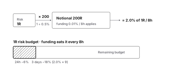
A tight 0.5% stop makes your notional roughly 200x your risk, so a 0.01% per-8h funding rate drains about 2.0% of 1R each stamp — near 18% over a three-day hold.
The most intuitive way to analyze this is by expressing funding in R units (where 1R represents the risk distance between entry and stop-loss). Let the stop-loss distance as a fraction of the entry price be:
$$SL_{frac} = \frac{|fill - sl|}{fill}$$
Since effective notional leverage is the inverse of this fraction, the cumulative funding paid over a holding period, expressed in R units, is:
$$\text{funding_R} = \frac{\text{direction_sign} \times \text{funding_rate} \times \text{periods}}{SL_{frac}}$$
Here, direction_sign is +1 for longs and -1 for shorts, reflecting the fact that long positions pay funding when the rate is positive, whereas short positions receive it.
A worked example (calculation, not a measurement)
Consider a breakout setup with a 0.5% stop-loss. This stop-loss fraction implies an effective notional leverage of approximately 200x ($\frac{1}{0.005}$).
- Under normal market conditions, Binance perpetual contracts typically publish a baseline funding rate of approximately 0.01% per 8-hour window.
- Per 8-hour window, this translates to a cost of $0.01% \times 200 = 2.0%$ of a single R unit.
- Holding the position for 24 hours spans three funding windows, meaning funding alone drains roughly 6% of 1R.
- Holding for three days spans nine windows, which accumulates to a funding drag of approximately 18% of 1R.
During strong trends, funding rates routinely expand to 0.03%–0.05% per window. At these levels, a 24-hour hold drains roughly 18%–30% of 1R, and a multi-day hold can easily exceed 50% of 1R. Since none of this drag appears in a backtest that ignores funding, a seemingly profitable equity curve can collapse the moment live positions are held across funding timestamps.
The solution is to deduct funding directly from each trade’s expectancy using the formula above. The implementation code is provided in Section 6.
3. Crypto graveyard #2: silent data gaps
Crypto markets trade 24/7. Consequently, the simplest method for historical data collection—looping queries to a single REST endpoint—is also the most vulnerable to data loss. API rate limits and transient connection drops can silently omit candles without raising runtime exceptions.
A missing candle is not merely a cosmetic issue. Rolling indicators (such as moving averages or ATR) shift along the time axis when bars are missing. As a result, a signal that fires at bar T in your backtest would, on complete data, have actually fired at T+k. Consequently, the strategy you are testing is no longer the strategy you deploy.
The remedy is to construct a three-tier data collection pipeline rather than relying on a single API loop:
- Monthly archive ZIPs for the vast majority of historical data (fast, complete, and immutable).
- Daily archive ZIPs to fill the gaps for recent weeks not yet covered by the monthly releases.
- Live REST queries exclusively for the trailing hours not yet archived.
Merge the three on a strict timestamp index, then assert that the bar count matches the expected count for the date range. Any gap that survives that assertion will silently corrupt a live trade.
4. The other three graveyards are universal, and we measured them elsewhere
The limit-fill illusion, execution slippage, and look-ahead bias are not unique to crypto; they degrade stock, FX, and traditional futures backtests in the exact same manner. Detailing them here would duplicate the empirical analysis already documented in our Backtest Autopsy series and dilute the citation authority of those research spokes. Therefore, we present only a concise summary paragraph for each, along with links to the corresponding studies.
Graveyard #3: The Limit-Fill Illusion
Standard backtest engines treat any candle wick touching your limit price as a guaranteed fill. In live trading, this assumption fails due to queue priority and spread dynamics. Furthermore, when both the stop-loss and take-profit targets lie within a single candle, the bar indicates that both levels were touched but cannot resolve the execution order. While requiring the price to penetrate the target level by ~0.2% is a common industry rule of thumb, it is merely a conservative heuristic rather than an empirical law. We analyzed the true execution probability inside a single candle, including same-bar execution order, in our dedicated study: read which hits first when stop-loss and take-profit share one candle. The related phenomenon where executing deeper fills acts as an adverse selection filter—capturing primarily losing trades—is analyzed in why your entry price is the edge.
Graveyard #4: Slippage and Latency
When a limit order misses and the engine falls back to a market order at the next bar’s open, the account pays taker fees and execution slippage instead of the maker assumptions baked into most backtests. In stressed regimes, that gap widens sharply. We modeled the maker-versus-taker expectancy gap and the slippage grid in the dedicated slippage spoke: see the slippage autopsy.
Graveyard #5: Look-Ahead Bias via Time-Series Joins
Merging external datasets (e.g., regime classifiers, correlation matrices) with historical bar data is a frequent source of look-ahead bias. Unless the join is strictly keyed on (timestamp, symbol), future labels can attach to historical bars, yielding an impossibly smooth, artificial equity curve. The exact mechanism, and how a single misaligned .shift() operation introduces this leakage, is dissected in look-ahead bias and the penetration trap.
5. The pitfall map
| Graveyard | Crypto-specific? | Symptom in live trading | Where it’s handled |
|---|---|---|---|
| Funding drag | Yes (perpetuals only) | Equity curve appears profitable, but bleeds once positions cross the 8h funding timestamp. | This guide, §2 + §6 code |
| Data gaps | Partly (inherent to APIs; severe in 24/7 crypto) | Indicators shift; signals fire on the wrong bar. | This guide, §3 |
| Limit-fill illusion | No (universal) | High simulated win rate; unexecuted or missed fills in live trading. | Autopsy: intrabar & entry-price spokes |
| Slippage & latency | No (universal) | Optimistic maker assumptions overstate the trading edge. | Autopsy: slippage spoke |
| Look-ahead via joins | No (universal) | Artificially smooth and unrealistic equity curve. | Autopsy: look-ahead spoke |
6. Python: deduct funding and friction in R units
This implementation corrects the two crypto-specific drags addressed in this guide. It expects trade-level rows and returns a net R-multiple that subtracts cumulative funding and execution friction, rather than merely logging them as informational columns.
import numpy as np
import pandas as pd


def apply_funding_and_friction(
    df: pd.DataFrame,
    taker_fee: float = 0.0004,
    slippage_pct: float = 0.0005,
) -> pd.DataFrame:
    """Adjust per-trade R-multiple expectancy for the two crypto-specific
    drags: notional funding cost and execution friction.

    Expected columns:
      entry_price, stop_loss_price,
      funding_rate (signed, per 8h window),
      funding_periods (count of 8h windows held),
      direction (+1 long, -1 short),
      gross_pnl_R (gross result in R units).
    """
    out = df.copy()

    # Stop distance as a fraction of entry price.
    # This fraction is the inverse of effective notional leverage,
    # so funding scales by 1 / sl_frac.
    out["sl_frac"] = (
        (out["entry_price"] - out["stop_loss_price"]).abs() / out["entry_price"]
    )
    out["sl_frac"] = out["sl_frac"].replace(0, np.nan).fillna(0.01)  # zero-division guard

    # Funding cost in R units, matching the body formula.
    # The direction sign is critical: a long pays when funding_rate > 0, whereas a short receives it.
    # A positive funding_cost_R means the trade LOSES that many R to funding.
    out["funding_cost_R"] = (
        out["direction"] * out["funding_rate"] * out["funding_periods"]
    ) / out["sl_frac"]

    # Execution friction (taker fee + slippage), expressed in R units.
    out["friction_cost_R"] = (taker_fee + slippage_pct) / out["sl_frac"]

    # Net expectancy actually deducts both drags.
    out["net_pnl_R"] = (
        out["gross_pnl_R"] - out["funding_cost_R"] - out["friction_cost_R"]
    )

    return out
This code resolves two critical bugs found in common open-source repositories: first, it incorporates the trade direction into the funding calculation (ensuring shorts receive funding when rates are positive); second, it computes and returns the net R-multiple directly instead of leaving the drags as unused columns.
For the limit-fill, slippage, and look-ahead remedies, use the engines described in the linked spokes rather than re-implementing them here.
7. FAQ
Q1. How much does funding actually cost a tight-stop scalper?
At a baseline 0.01% per 8-hour funding rate, a 0.5% stop-loss implies approximately 200x effective leverage, meaning each funding timestamp costs roughly 2.0% of 1R. A 24-hour holding period (3 timestamps) costs about 6% of 1R, while a three-day hold (9 timestamps) drains about 18% of 1R. During strong trends, funding rates can expand to 0.03%–0.05% per timestamp, multiplying these costs by three to five times. Note that these figures are mathematical calculations derived from explicit assumptions, not empirical backtest results. The mechanics and 8-hour scheduling of perpetual funding are documented in Binance Academy’s funding-rate primer.
Q2. What is the basis for the 0.2% price penetration rule?
It is a conservative industry rule of thumb, not an empirical constant. Treating every wick touch as a guaranteed fill overstates the execution rate; requiring a minor penetration before confirming a fill serves as a realistic safeguard. The exact execution sequence inside a candle (resolving whether the stop-loss or take-profit hits first) is analyzed in the intrabar study.
Q3. Why model slippage as a grid rather than a flat fee?
A flat fee is blind to tail risk. Bid-ask spreads widen sharply during news events and liquidity crises, so sweeping slippage across a range reveals whether the strategy survives stressed regimes or only calm ones. The measured maker-versus-taker gap is in the dedicated slippage spoke.
Q4. How can I prevent look-ahead bias during data merging?
Ensure all merge operations are strictly keyed on (timestamp, symbol), validate the row count post-merge via assertions, and shift any external feature columns forward by one bar (.shift(1)). This ensures the backtest engine only references historical, closed bars. The prevention architecture is fully dissected in the look-ahead spoke.
Q5. Are the numbers presented in this guide empirical?
No, the funding metrics are arithmetic projections derived from explicit assumptions (funding rate, stop-loss size, and holding period). While mathematically reproducible, they are not empirical. All measured statistics within this research cluster are sourced from the respective Backtest Autopsy spokes, each utilizing its own distinct historical dataset and sample size.
Related research
- 7 Ways Your Backtest Is Lying to You (Measured, Not Guessed) — the hub guide tying all seven measured failure modes together
- Which hits first when stop-loss and take-profit share one candle
- Why your entry price is the edge
- Look-ahead bias and the penetration trap
- Correlation is not a direction signal
- Quant Strategy Research hub
Updates & changelog
- 2026-06-04: Restructured the document into a methodology guide. Retained the two crypto-specific graveyards (funding drag and data gaps), providing a corrected R-unit funding formula and net-expectancy Python code. Delegated the three universal graveyards to their respective Backtest Autopsy spokes. Removed unverified statistics and any fabricated source attributions.
Educational content only — not investment or financial advice. Data, prices, and tool specifications change; verify independently and paper-trade before risking capital.